章节
引言
过程描述
如何编码?
总结
使用TensorFlow进行线性回归
这篇教程是关于如何通过TensorFlow训练一个线性模型来拟合数据。或者,您可以查看这篇博文。
引言
在机器学和统计学上,线性回归是对诸如一个变量Y和至少一个作为自变量X之间关系的建模。在线性回归中,线性关系将由一个参数可通过数据进行估计的预测函数进行建模,并称为之线性模型。线性回归算法的主要优点是简单易用,使用它可以非常直接地解释新的模型,并将数据映射到新的空间。在这篇文章中,我们将会介绍如何使用TensorFlow来训练线性模型以及如何展示生成的模型。
过程描述
为了训练这个模型,TensorFlow循环遍历数据,它应该找到一条拟合数据的最佳直线(因为我们使用的是线性模型)。通过设计一个合适的优化算法其要求是一个合适的损失函数来预计两个变量X,Y之间的线性关系。数据集可以从Stanford course CS 20SI:TensorFlow for Deep Learning Research下载。
如何编码?
首先,第一步加载所需要的库和数据集。
# Data file provided by the Stanford course CS 20SI: TensorFlow for Deep Learning Research.
# https://github.com/chiphuyen/tf-stanford-tutorials
DATA_FILE = "data/fire_theft.xls"

# read the data from the .xls file.
book = xlrd.open_workbook(DATA_FILE, encoding_override="utf-8")
sheet = book.sheet_by_index(0)
data = np.asarray([sheet.row_values(i) for i in range(1, sheet.nrows)])
num_samples = sheet.nrows - 1

#######################
## Defining flags #####
#######################
tf.app.flags.DEFINE_integer(
    'num_epochs', 50, 'The number of epochs for training the model. Default=50')
# Store all elements in FLAG structure!
FLAGS = tf.app.flags.FLAGS
接着我们定义和初始化所需要的变量。
# creating the weight and bias.
# The defined variables will be initialized to zero.
W = tf.Variable(0.0, name="weights")
b = tf.Variable(0.0, name="bias")
之后,我们定义一些必要函数。不同的标签用于区分定义的函数。
def inputs():
    """
    Defining the place_holders.
    :return:
            Returning the data and label lace holders.
    """
    X = tf.placeholder(tf.float32, name="X")
    Y = tf.placeholder(tf.float32, name="Y")
    return X,Y
def inference(X):
    """
    Forward passing the X.
    :param X: Input.
    :return: X*W + b.
    """
    return X * W + b
def loss(X, Y):
    """
    compute the loss by comparing the predicted value to the actual label.
    :param X: The input.
    :param Y: The label.
    :return: The loss over the samples.
    """

    # Making the prediction.
    Y_predicted = inference(X)
    return tf.squared_difference(Y, Y_predicted)
# The training function.
def train(loss):
    learning_rate = 0.0001
    return tf.train.GradientDescentOptimizer(learning_rate).minimize(loss)
接下来,我们遍历不同代的数据,并执行优化过程。
with tf.Session() as sess:

    # Initialize the variables[w and b].
    sess.run(tf.global_variables_initializer())

    # Get the input tensors
    X, Y = inputs()

    # Return the train loss and create the train_op.
    train_loss = loss(X, Y)
    train_op = train(train_loss)

    # Step 8: train the model
    for epoch_num in range(FLAGS.num_epochs): # run 100 epochs
        for x, y in data:
          train_op = train(train_loss)

          # Session runs train_op to minimize loss
          loss_value,_ = sess.run([train_loss,train_op], feed_dict={X: x, Y: y})

        # Displaying the loss per epoch.
        print('epoch %d, loss=%f' %(epoch_num+1, loss_value))

        # save the values of weight and bias
        wcoeff, bias = sess.run([W, b])
在上面的代码中,sess.run(tf.global_variables_initializer())初始化所有定义的全局变量。train_op建立在train_loss之上,并将在每一步中被更新。最后将返回该线性模型的参数,例如wcoff和bias。为了评估,我们将演示预估直线和原始数据是怎么样让模型去拟合数据的。
###############################
#### Evaluate and plot ########
###############################
Input_values = data[:,0]
Labels = data[:,1]
Prediction_values = data[:,0] * wcoeff + bias
plt.plot(Input_values, Labels, 'ro', label='main')
plt.plot(Input_values, Prediction_values, label='Predicted')

# Saving the result.
plt.legend()
plt.savefig('plot.png')
plt.close()
结果如下图所示:
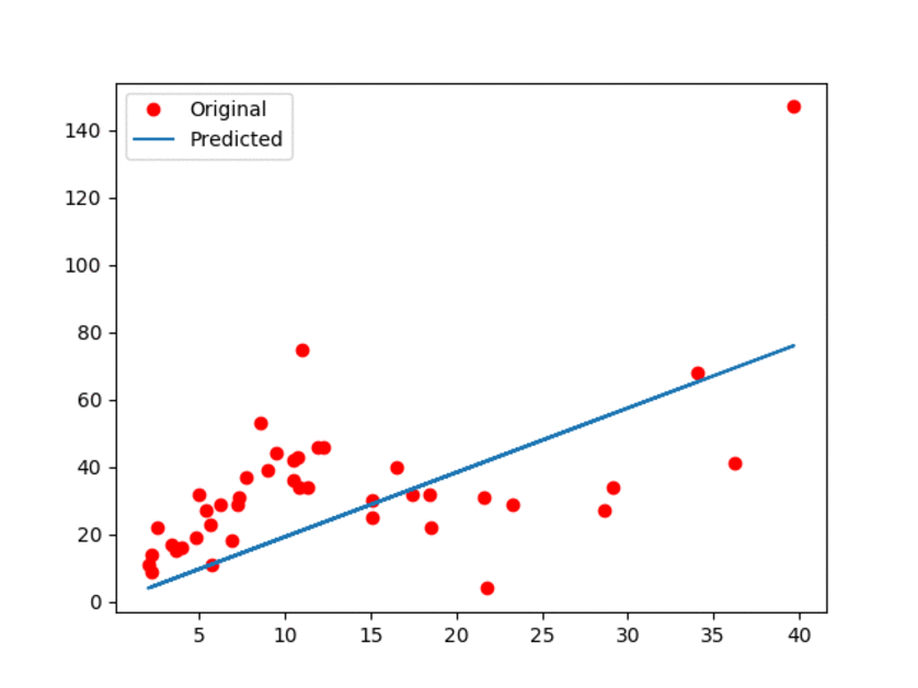 图1:原始数据和预估线性模型
在上面的GIF动画中,展示了更新过程中模型中有一些小偏差。可以观察到,线性模型肯定不是最好的。然而,我们提到过,它的优势就是简单易用。
总结
在本教程中,我们使用TensorFlow完成了线性模型创建。在训练后得到的直线并不能保证是最好的。不同的参数会影响收敛精度。使用随机优化找到线性模型,其简单性使我们的世界变得更容易。